
Report section
3.4 Sensitivities
3.4.1 Random temporal variation
- Regardless of climate change, the weather changes randomly (effectively) from year to year. That affects not only temperatures, but also the profile and average intensity of wind and insolation. To a lesser extent, there are also small differences in human aggregate behaviour. To test this, we can check how this scenario would look under the conditions that pertained in 2016 and 2018 (our base scenario used 2017 conditions). All three years were slightly milder than average, but not exceptionally mild. They are adequate (and must be, given the constraints on the availability of real-world data) to test variations primarily in the timing rather than in the normality of the weather.
- Even with neighbouring years, there are some differences that make the data not perfectly comparable. In particular, wind and solar were being rolled out apace in this period. A fair amount of it was embedded. That means that embedded renewables had a bigger impact on electricity demand data in 2018 than in 2016. We use the demand data to estimate the profile rather than the amplitude, so it does not affect the totals. But embedded intermittents will have somewhat increased the apparent variations in demand in 2018 compared to 2016.
- As one would expect in years of non-exceptional weather, the temporal variation did not make much difference to the modelled aggregate electricity demand.
| 2016 | 2017 | 2018 |
|---|---|---|
|

|

|
- The variation in the demand profile is not easy to spot without the supply side to compare with it.
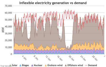
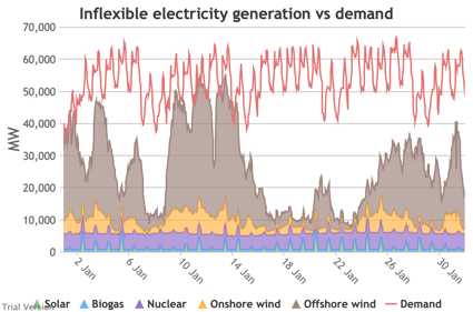
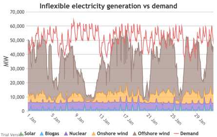
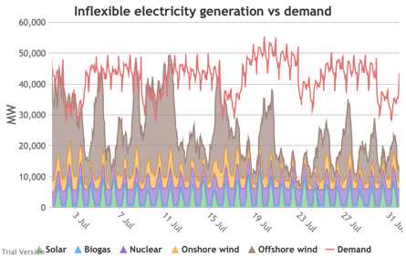
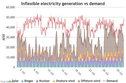
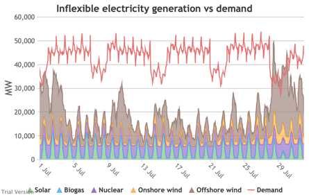
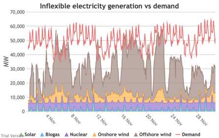
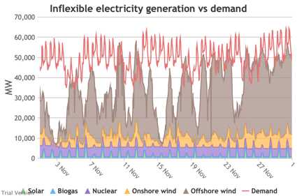
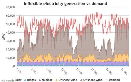
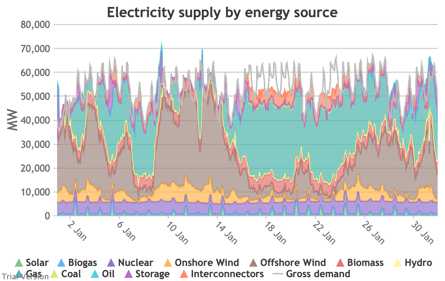
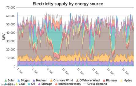
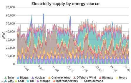
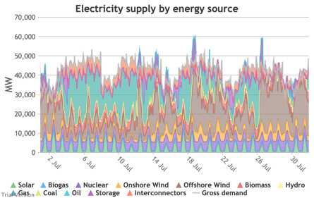
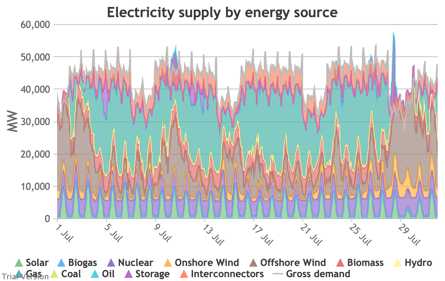
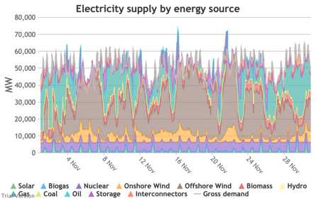
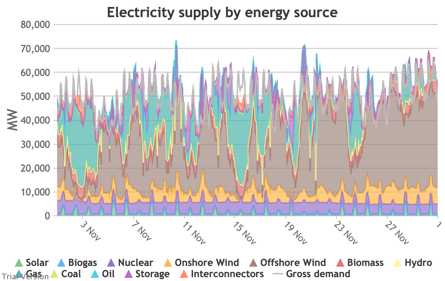
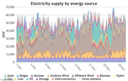
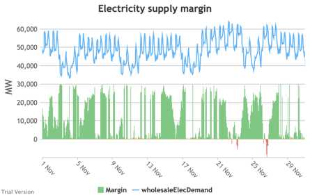
- The comparison of inflexible generation with wholesale demand shows more variation.
| 2016 | 2017 | 2018 |
|---|---|---|
|
|
|
|
|
|
|
|
|
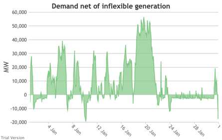
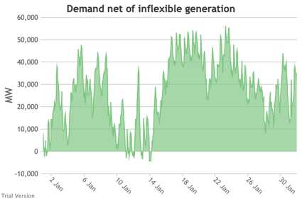
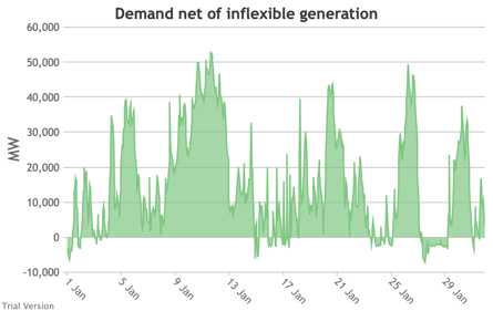
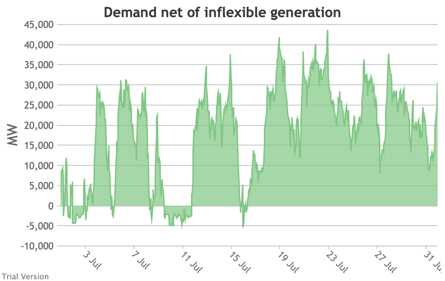
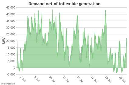
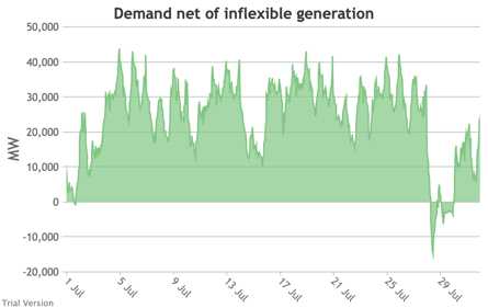
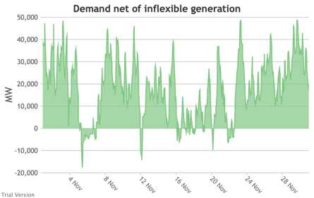
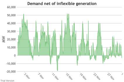
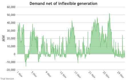
- That translates into significant variation in the demand net of inflexibles.
| 2016 | 2017 | 2018 |
|---|---|---|
|
|
|
|
|
|
|
|
|
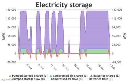
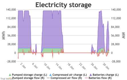
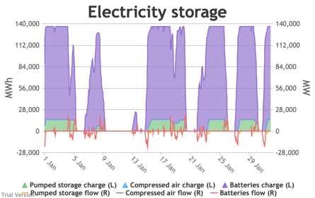
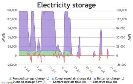
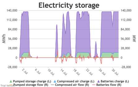
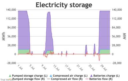
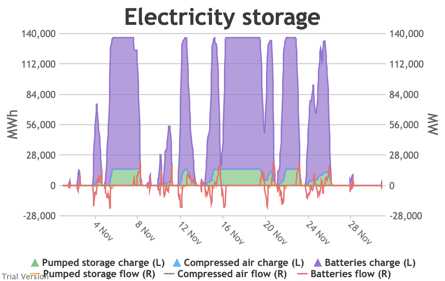
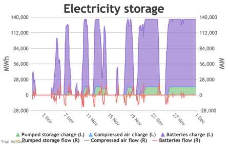
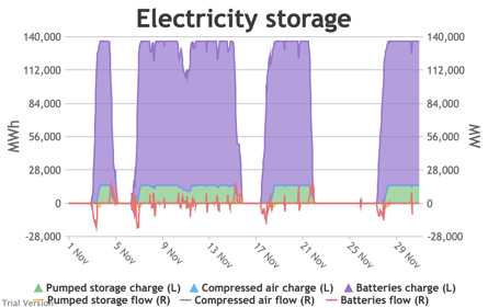
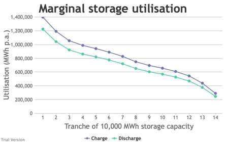
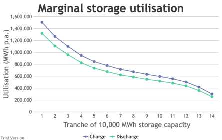
- That puts different strains on the storage capacity, and on its marginal use.
| 2016 | 2017 | 2018 |
|---|---|---|
|
|
|
|
|
|
|
|
|
|

|
|
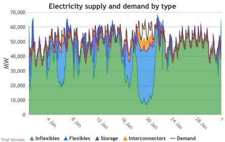
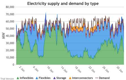
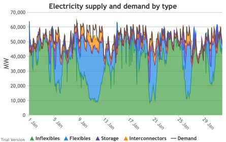
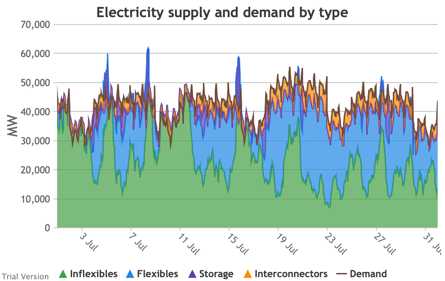
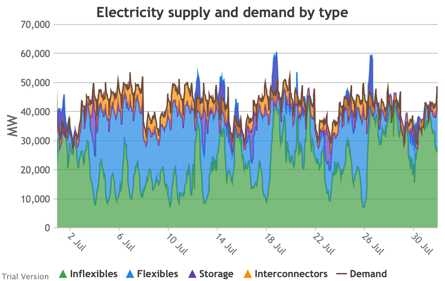
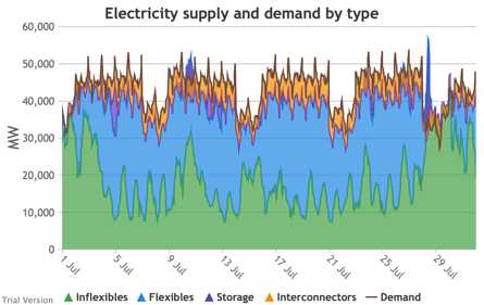
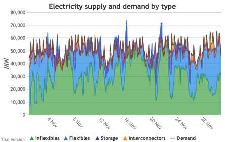
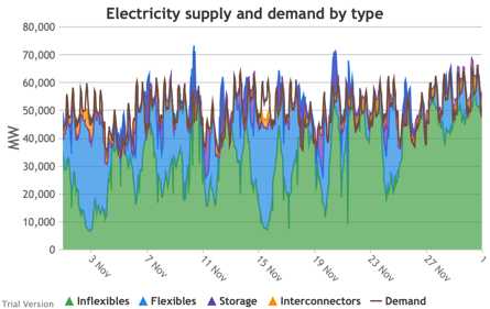
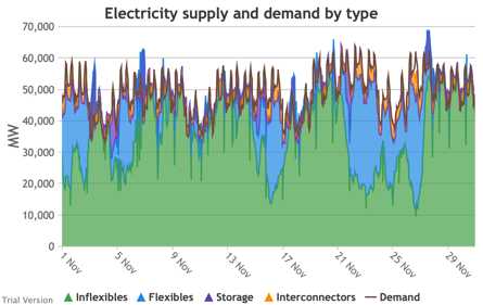
- Interconnector flows also have to vary. The net effect on supply by type is:
| 2016 | 2017 | 2018 |
|---|---|---|
|
|
|
|
|
|
|
|
|
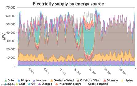
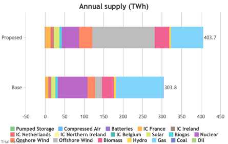
- Likewise, the net effect on supply by source (i.e. technology) is:
| 2016 | 2017 | 2018 |
|---|---|---|
|
|
|
|
|
|
|
|
|
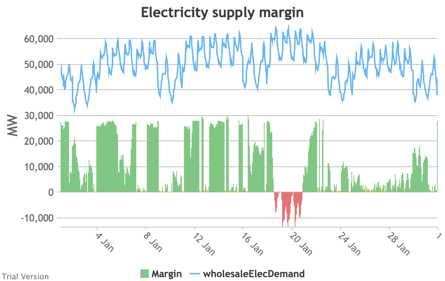
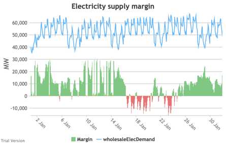
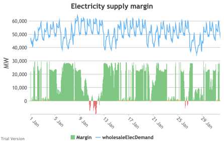
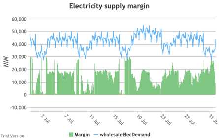
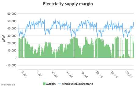
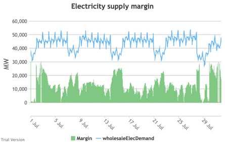
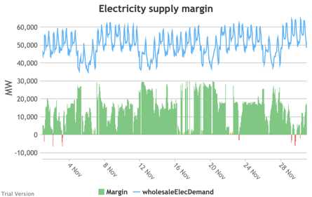
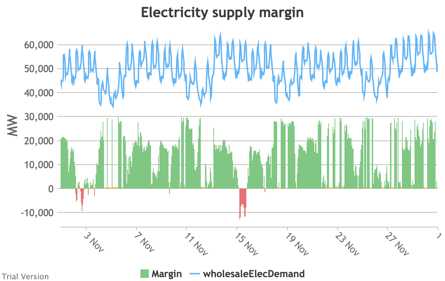
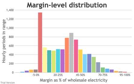
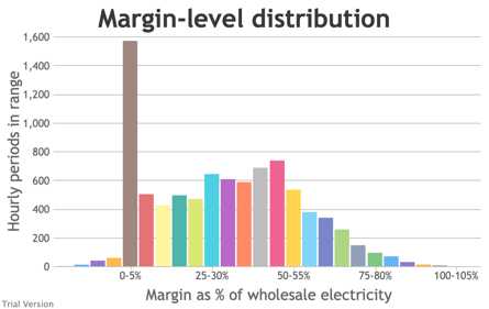
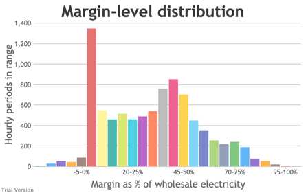
- That feeds through to the electricity supply margin.
| 2016 | 2017 | 2018 |
|---|---|---|
|
|
|
|
|
|
|
|
|
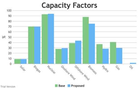
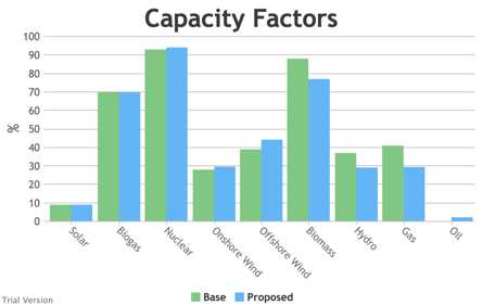
- This adds up to small differences in aggregate technology utilisation, but material differences at the margins.
| 2016 | 2017 | 2018 |
|---|---|---|

|

|
|
|
|

|
|
|
|
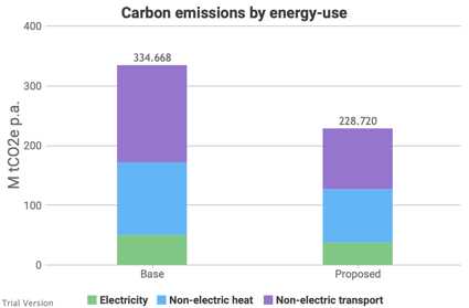
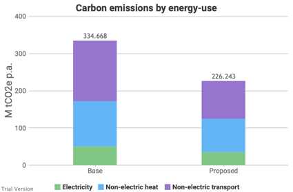
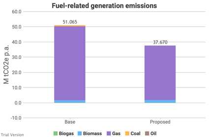
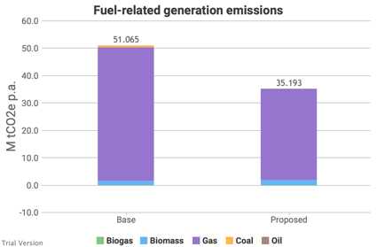
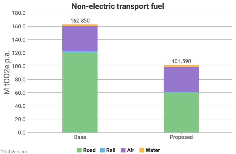
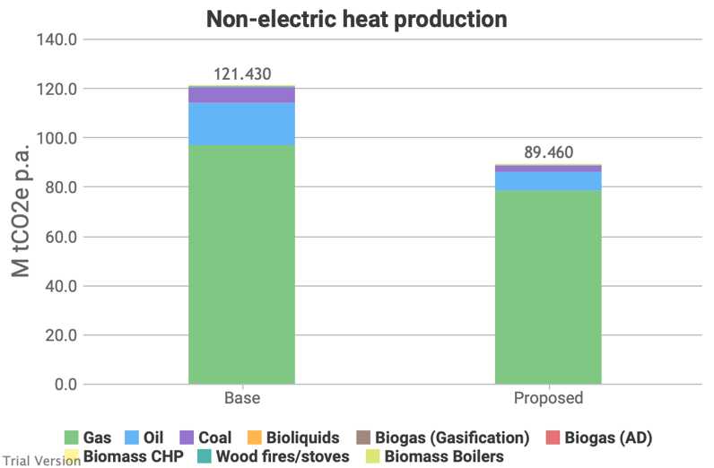
- Because this system still relies on fossil fuels to a significant extent, the carbon footprint of the energy system varies from year to year.
| 2016 | 2017 | 2018 |
|---|---|---|
|

|
|
|

|
|
|
|
|
|
|
|
The differences are quite small, because the nature of this comparison is the same spread of technologies and roughly similar levels of aggregate demand in the various uses. The main change in the inputs is the profile, which has a bigger bearing operationally than on the cumulative outcome. In the case of non-electric heat and transport emissions, it’s an artefact of the model design that there is no difference between these projections without a change in the aggregate.
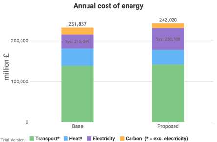
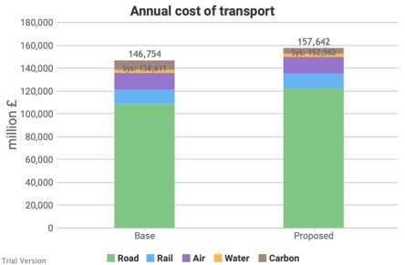
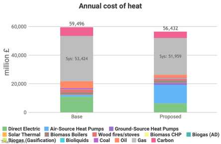
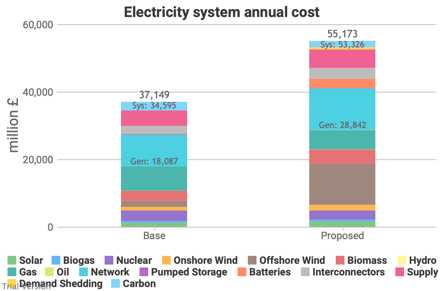
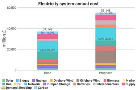
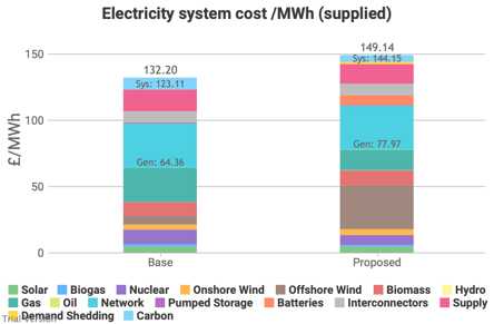
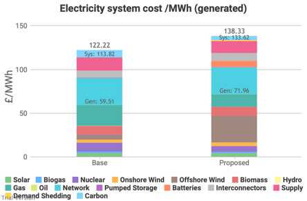
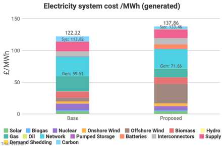
- 3.4.1.13 Costs also vary marginally from year to year depending on the impact of the weather on the profiles of supply and demand.
| 2016 | 2017 | 2018 |
|---|---|---|

|

|
|

|

|
|

|

|
|
|

|
|

|

|
|

|
|
|
These changes are small enough that they are mainly useful as demonstration that the model is recalculating for the variations, but not over-reacting.