
Report section
3.3.6 Electricity storage and level of charge
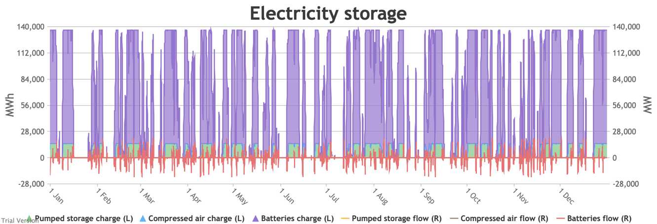
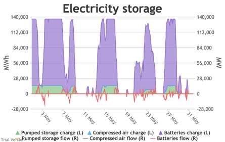
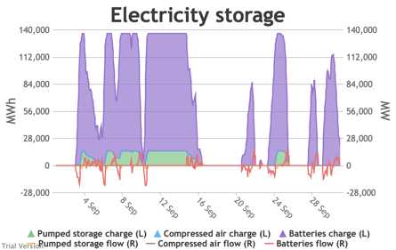
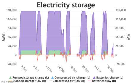
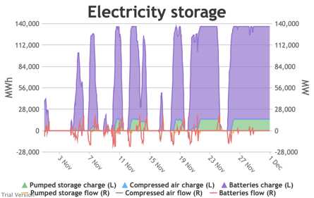
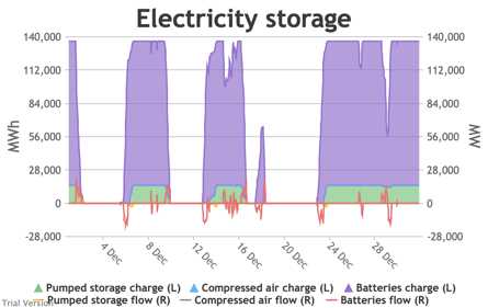
These charts show the flows into and out of storage (the lines) and the level that they are charged to (the areas) in each period.
|
||

|
|
|
|
|
|
|
|
|
|
|
|
- We put 20 GW / 120 GWh of new battery storage into the model (on top of the modest existing pumped-hydro and battery storage) to test how it would handle these conditions. To maximise its value, the model assumes it is the first option for balancing, before interconnectors and flexible generation.
- This requires a bit more explanation than previous charts:
- Storage has two constraints: (a) the amount of energy (MWh) it can hold, and (b) the maximum rate (MW) at which that energy can flow into or out of the storage unit.
- is bounded by the energy capacity at one end, and zero at the other (i.e. can’t have less than no energy in it, nor more energy in it than it can hold).
- is roughly centred on zero, with flows into storage represented by negative numbers (i.e. this is from a system perspective, so flows into storage are flows out of the system), and flows out of storage represented by positive numbers (i.e. the storage is adding to the energy in the system).
- The model assumes that the storage units will take any of the excess from the previous section, limited by (a) the maximum flow-rate (to simplify things, we make the unsound assumption that the maximum inflow- and outflow-rates are the same), (b) the storage capacity (i.e. it stops taking electricity when it is full), and (c) an internal priority list between storage technologies, which assumes that batteries take priority over compressed air (because a key purpose of compressed air is to provide better economics for longer-term storage than batteries), and compressed air takes priority over pumped storage (because pumped-storage costs are largely sunk – this is not a strong generalisation and could well not be reflected in real-life operation). In this scenario, we have not yet assumed any compressed air storage, so the priority is simply that batteries take excess power in priority to pumped storage (which is anyway dwarfed by the assumed battery capacity).
- Conversely, the model assumes that the storage units will supply any net demand (from the previous section) in priority to interconnectors and flexible generation, limited (as before) by (a) the maximum flow-rate, (b) the storage capacity, and (c) the priority order between storage technologies. Again, these assumptions may not be reflected in real-life operation, where priority will be determined by commercial decisions.
- We have to take account of round-trip losses at some point. The model assumes that the storage capacity (MWh) reflects capacity after losses, and that the losses occur before the electricity is stored. For example, if the technology’s round-trip efficiency were 80% (i.e. 20% round-trip losses), its capacity were 100 MWh, and its maximum flow-rate were 10 MWh, it would take 12.5 hours at full flow to fully charge the unit, but only 10 hours to discharge. This is almost certainly not how it works in practice, but it is largely semantic and simplifies the calculations. The end result should be the same as if we had made a more specific allocation of losses before and after storage. The main difference would be the notional capacity.
- The chart shows the flows as discrete lines (with the scale on the right) and the stored energy as stacked areas (with the scale on the left vertical axis).
- Remember that we deliberately specified storage with a conventional ratio of capacity (MWh) to power (MW) designed for the economically-optimal operational profile of frequent, regular charge/discharge cycles (typically once or twice a day). That has produced a usage profile with reasonably-high frequency. But it is nowhere near the ideal frequency and regularity because it is responding to a highly-irregular supply/demand pattern.
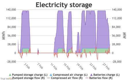
- For example, the period of 16-24 Jan discussed above appears in the storage chart as a gap.
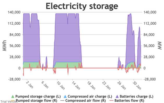
Even 120 GWh of electricity storage is used up within a day on 15 Jan, as the wind dies down and the demand net of inflexibles becomes substantial. It remains substantial for 8 days. It cannot supply anything in that period because it is empty. It does not charge up again because there is pressure on the swing suppliers (flexible generators and interconnectors) and it would be counterproductive and expensive to buy electricity when marginal costs are high. So it waits until 26 Jan to start re-charging, when the wind has strengthened and net demand is lower. - Such circumstances are not uncommon. Theoretically, storage technologies could continue to charge and discharge if there is some supply margin between the flexible generators and interconnectors. But round-trip losses mean that storage loses money if there is not a material price gap between purchase and sale. Such a margin relies on material differences in the tightness of the market. It does not make sense for storage to charge and discharge when there is little difference in purchase and sale price because the tightness of the market is not varying sufficiently, even though it would be theoretically possible to do so. The frequency and scale of the swings in market tightness are a material difference between current conditions and the modelled conditions under heavy electrification. It is the effect of increased irregularity because of (a) the penetration of wind and (to a lesser extent) solar, and (b) the less-regular demand profile for heat.
- A marginal analysis shows the decreasing returns to scale.
- In reality, one would not install most of these tranches, unless the costs of storage were dramatically lower than they are currently, or the value of balancing services were dramatically higher. We estimate that the cost of battery storage at this scale is around £280/MWh, which is an order of magnitude more than it would generally be thought to be worth.
- And yet this is at a scale that can address only a small proportion of the discrepancy between demand and inflexible output, aiming to deal primarily with short-period variations. If we wanted to deal with longer-period variation (e.g. seasonality) through storage, the utilisation would be much lower than even the last tranche in the chart above. The cost would be in the thousands of pounds per MWh.
- Other technologies such as compressed air storage may lower that somewhat. They claim to reduce the capital cost per MWh of having a higher ratio of MWh to MW and thereby reduce the cost of somewhat longer-term storage. But it is noticeable that their example applications still hope (in the first instance) to be high frequency. They cannot overcome the fundamental relationship between frequency-of-use and economic return, just marginally reduce the impact of lower frequency.
- The reality of storage is that it is best-suited to high-frequency, regular patterns of use, and is ill-suited to addressing the irregular profiles generated by this scenario.

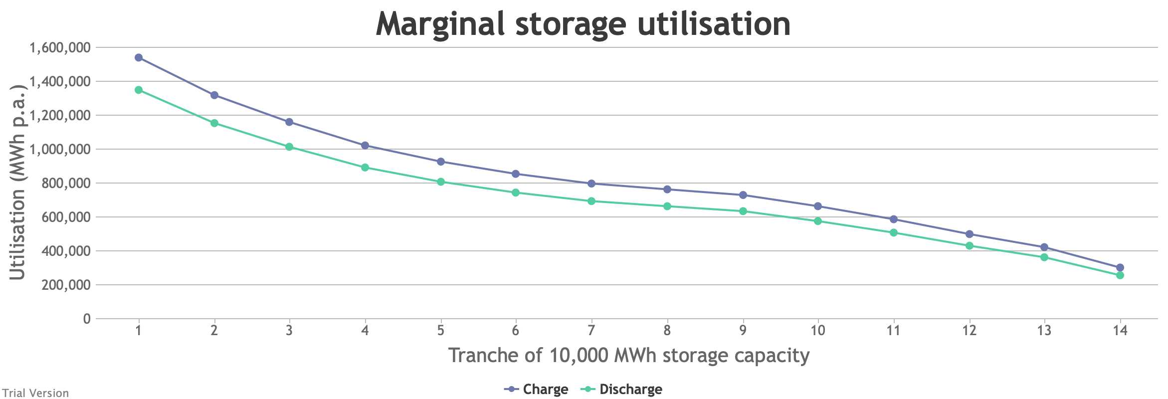
The storage capacity (in MWh, not MW) in this scenario is divided into notional tranches of 10 GWh (120 GWh of new battery storage, plus the modest existing capacity of pumped storage and batteries). If we had only installed 10 GWh of storage, the opportunities to charge/discharge would have amounted to annual sales of 1.35 TWh. Even that is significantly worse (equivalent to one full discharge just under every 3 days) than the almost-daily opportunities currently available to Dinorwig etc. But this falls quite sharply as we add capacity. The 4th tranche only has opportunities to discharge 891 GWh p.a., equivalent to one full discharge every 4 days. The last tranche is down to 256 GWh p.a., or one discharge every 14 days.